How to Create a Pivot Table in Excel: A Practical Guide

Excel pivot tables summarize large datasets into structured reports with only a few steps.

For example, if your sales team has accumulated a year's worth of data and your manager requests a monthly sales by region summary, a pivot table can generate it instantly.

What is an Excel Pivot Table? How It Differs from Regular Tables

Regular Excel tables have a fixed structure where each row records individual transactions and each column represents fields like date, region, product name, and amount. In contrast, Excel pivot tables are dynamic summary tools that reference source data to automatically calculate sums, counts, averages, and maximum values. Instead of manually writing Excel formulas like SUM, AVERAGE, SUMIF, or AVERAGEIF, you simply drag fields into row, column, and value areas—Excel handles the aggregation automatically.

With the same dataset, placing Month in Rows and Region in Columns shows monthly sales by region. Reversing the arrangement changes the perspective without altering the source data.

When source data changes, a single pivot table refresh updates everything to reflect the latest information. Converting the pivot table data source to table format enables automatic range expansion.

Excel Pivot Table Tutorial: Basic Steps for Beginners

Creating an Excel pivot table is simpler than you think.

1. Select Data Range
Click any cell within your source data and press Ctrl+A to select the entire range.

2. Insert Pivot Table
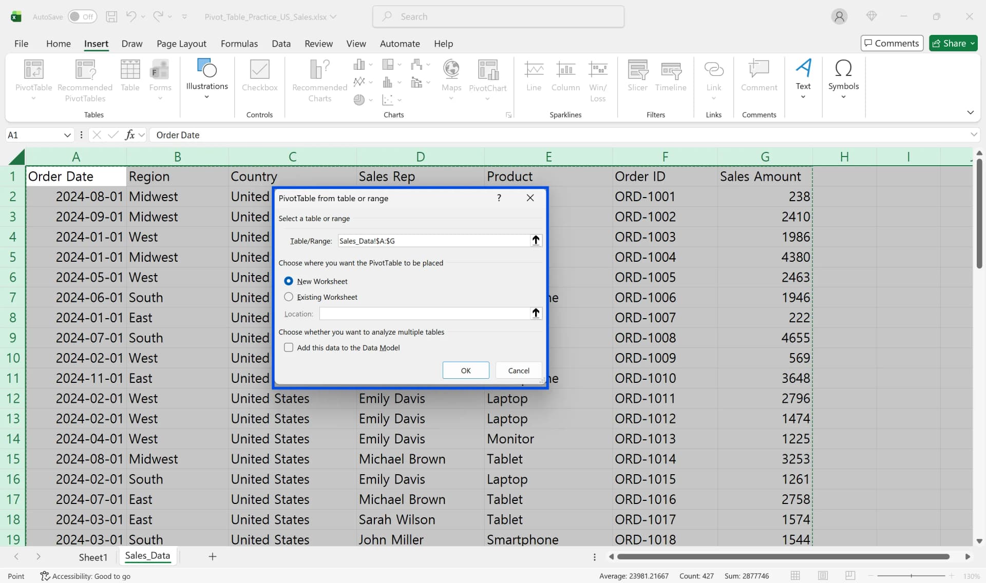
Go to the [Insert] tab → Click [PivotTable] → Select "New Worksheet"

3. Drag and Drop Fields
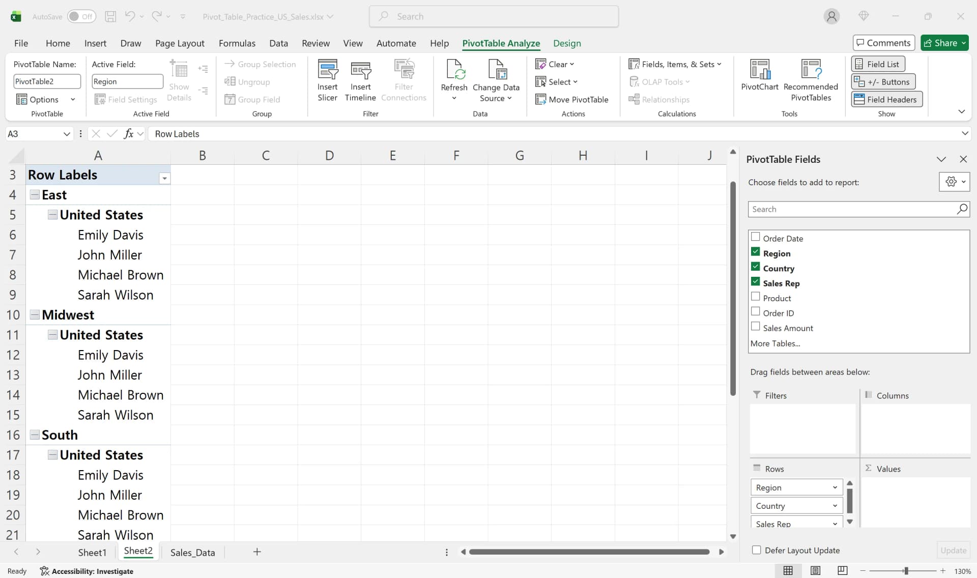
When the new sheet opens, you'll see an empty pivot area on the left and the PivotTable Fields pane on the right. Drag fields like "Region," "Month," "Product Name," and "Sales Amount" into the Rows, Columns, Values, or Filters areas. For example, placing Region in Rows, Month in Columns, and Sales Amount in Values automatically creates a Region × Month sales summary table.

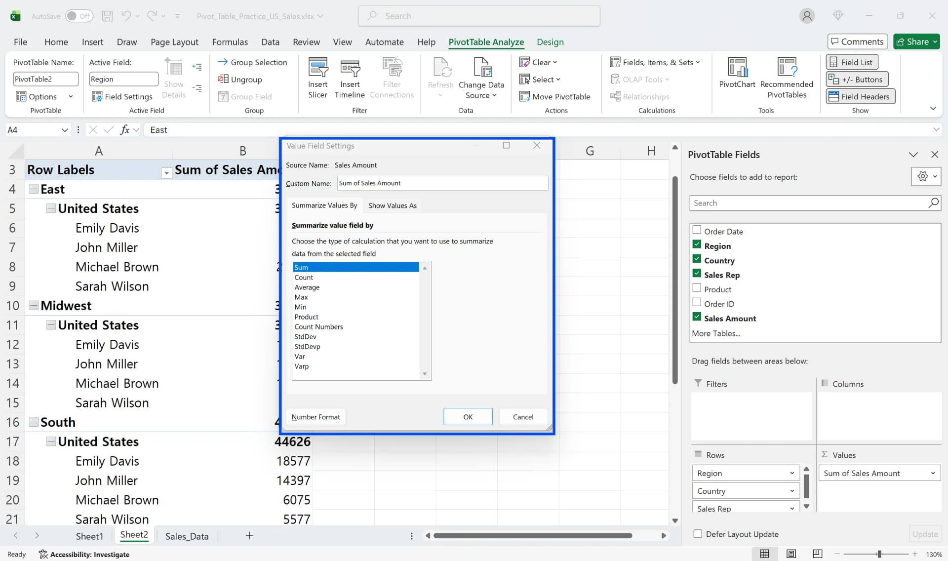
4. Adjust Value Field Settings
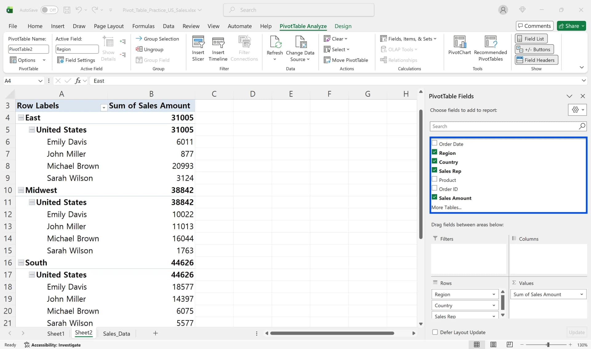
Click on the value field to open the [Value Field Settings] menu, where you can change the summary method to Sum, Count, Average, Max, or Min. Number fields default to Sum, but Excel may auto-select Count if text is mixed in or many cells are empty. The pivot table handles functions like COUNT and AVERAGE automatically—no manual formulas needed.

Common Excel Pivot Table Setup Mistakes Beginners Miss

The most common mistake when creating a pivot table is having blank rows or columns in the source data. When you press Ctrl+A, Excel may stop selecting at blank areas, which results in missing regions or periods in the pivot output. Before inserting a pivot table, remove blank rows and columns or manually confirm the full data range.

Another frequent issue is missing or duplicate column headers, which triggers the "Invalid field name" error. Ensure every column has a unique header in the first row (Date, Region, Product, Amount, etc.) before creating the pivot table.

Finally, placing numeric fields such as Sales Amount in the Row or Column area instead of the Values area prevents aggregation. Numeric fields must be placed in the Values section to calculate sums or averages correctly.

Why Pivot Table Refresh Not Working After Adding Data

When you create an Excel pivot table with a fixed range like A1:D100, any data added beyond row 101 won't be included in the source. This explains why your source sheet shows January 2025 data but the pivot table still shows data only through December. Here's how to fix it:

Method 1. Update Pivot Table Data Source (Temporary Fix)

1. Click any cell inside the pivot table
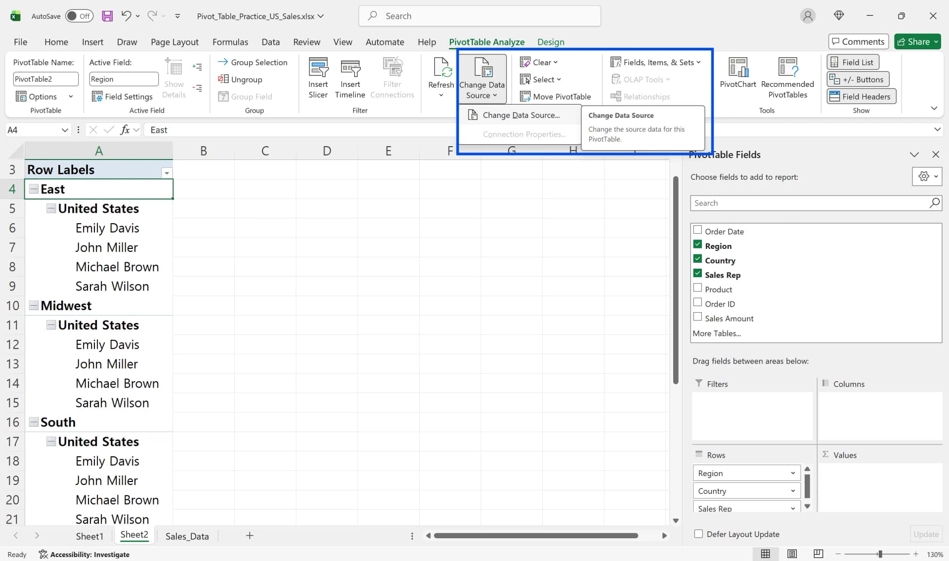
2. Go to the [PivotTable Tools] → [Analyze] tab → Click [Change Data Source]
3. Drag to include new rows, updating the range to A1:D200 (or your desired range), then click OK

Method 2. Pivot Table Refresh (For Value Changes Within Range)

If only values within the existing range have changed, you don't need to modify the pivot table data source—just refresh the pivot table.

1. Select a pivot cell, right-click → Choose [Refresh]
2. Or click the [Refresh] button in the [Analyze] tab
3. Keyboard shortcut: Alt+F5 (Alt+Ctrl+F5 to refresh all pivot tables simultaneously)

Method 3. Manage Source as Table Format (Permanent Solution)

1. Select source data range
2. Go to the [Insert] tab → Click [Table] or press Ctrl+T
3. Confirm "My table has headers" and click OK

Converting to table format makes the range automatically expand when adding new rows below, and any Excel pivot tables referencing this table will reflect new data with just a refresh. Table format also improves basic features like formatting, filtering, and sorting, making data management much easier before creating pivot tables.

Why Pivot Table Values Incorrect Compared to Source Data

If a value field appears numeric but is stored as text or contains many blank cells, Excel may default to Count instead of Sum. This explains why you might see 120 (record count) instead of a total sales amount such as 300,000. Open Value Field Settings and switch the summary method to Sum, or convert the source column to a numeric format before refreshing.

Duplicate records in the source data can also inflate totals. Use Remove Duplicates, COUNTIF, or Conditional Formatting to identify repeated transactions before rebuilding the pivot table.

Active filters or slicers may also cause discrepancies. If specific regions or months are selected, the pivot table summarizes only filtered data. Reset filters to “Select All” before comparing totals with the source sheet.

Excel Pivot Table Best Practices: Maintaining Stability in Real-World Use

When starting new projects, first convert the data input sheet to table format (Ctrl+T), then create pivot tables based on this table. Adding daily or monthly data rows automatically expands the source range, and a pivot table refresh instantly reflects the latest data. Make refreshing pivot tables a routine whenever you modify, delete, or add source values. To refresh multiple pivot tables at once, use the Refresh All function in the [Data] tab or press Alt+Ctrl+F5. In many reporting scenarios, pivot tables are more efficient than building complex summary formulas manually.

When reviewing reports, first check filter icons and slicer states at the top of the Excel pivot table. Pivot tables recognize fields based on header names and column structure, so inserting or deleting columns mid-structure can cause field recognition errors. In practice, separating analysis source sheets from reporting format sheets and keeping source structure as fixed as possible ensures stability.

Frequently Asked Questions About Excel Pivot Tables

Q. How to calculate percentages in Excel pivot tables?

Click on the value field → [Value Field Settings] → Under [Show Values As], select "% of Column Total" or "% of Grand Total"

Q. Does copying an Excel pivot table break the source connection?

Copying a pivot table within the same workbook preserves pivot functionality. However, if you paste a pivot table into a different workbook, it creates a separate cache with no link to the original source. In that case, go to the [PivotTable Analyze] tab and use [Change Data Source] to reconnect it to the correct range.

Q. How to group dates by month or quarter in pivot tables?

Place the date field in Rows or Columns → Right-click → Select [Group] → Choose month, quarter, or year units

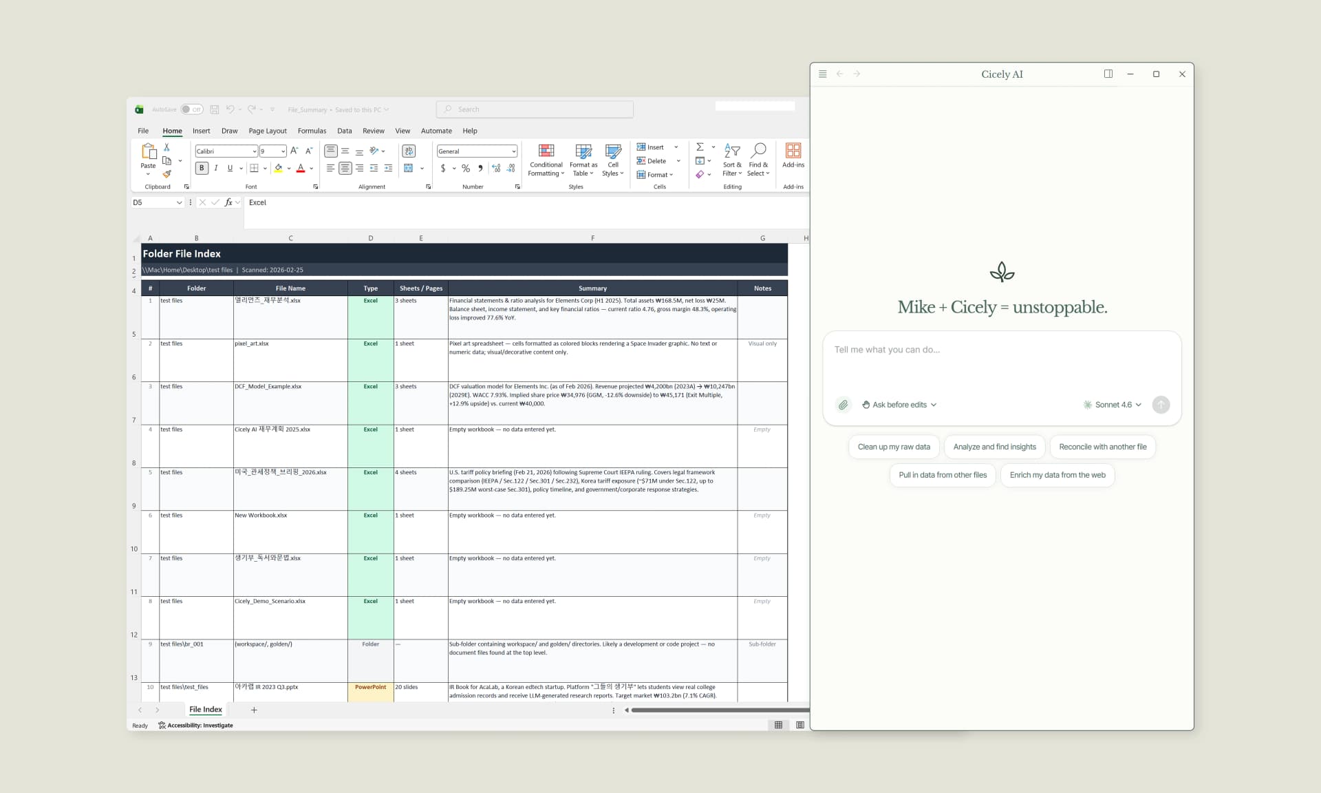
Work More Efficiently in Excel with Cicely AI

Building pivot tables often involves repeated adjustments such as refreshing data, fixing field placement, and correcting aggregation settings.

Cicely AI is a desktop-native AI coworker built for spreadsheet workflows. Instead of navigating menus manually, you can describe what you need in plain English, such as:

"Create a monthly sales pivot from this dataset."
"Refresh all pivot tables and reset filters."
"Fix this pivot table that is counting instead of summing."

Cicely reviews your worksheet structure and guides you through practical setup steps. Everything runs locally on your PC. No file uploads. No browser tools.