How to Link Data Between Sheets in Excel

It's Monday morning, and you need to compile sales data from multiple branches. North, South, and West each have their own sheet, and you need totals on a summary sheet. Copying and pasting between sheets wastes time and introduces errors.

Excel's cross-sheet references automate this. Use the right method (direct references, INDIRECT, or lookups) to reduce consolidation time while minimizing copy-paste errors. This guide shows you how to reference another sheet in Excel and fix common errors.

Why Reference another sheet in Excel?

Cross-sheet references link data automatically. Change the source, and formulas update instantly.

Most Excel workbooks split data across sheets: monthly sales, department budgets, project updates. It's easier to view and manage this way.

But when you need a report or dashboard, everything has to come together in one place. Opening each sheet to copy values is slow and risky. If the source data changes, you have to copy everything again.

Sheet references keep your formulas automatically in sync with the source.

How to Get Values from Another Sheet in Excel: Basic Methods

Direct references are the simplest way to pull data from another sheet.

Excel Formula to Reference Another Sheet (Direct Method)

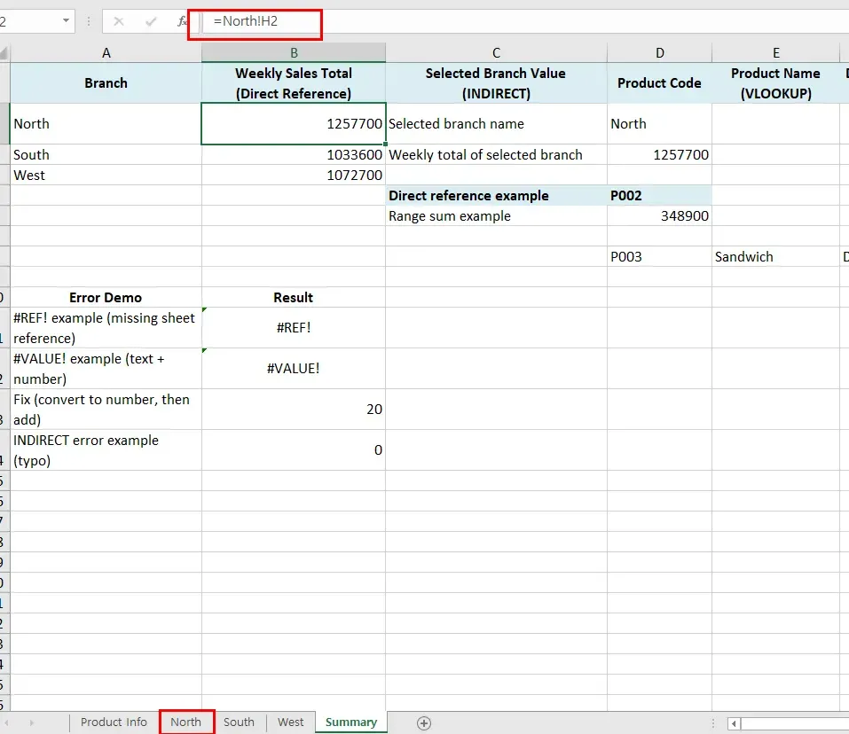
The formula is: =SheetName!CellAddress

For example, to get the value in cell H2 from sheet North:

1. Select the cell where you want the value.
2. Type =North!H2.
3. Press the Enter key.

North's H2 value appears in your cell. Change the referenced sheet, and your formula updates automatically.

How to Reference a Range from Another Sheet in Excel

To reference a range instead of a single cell, use the same method:

=SUM(North!E2:E10)

This grabs E2 through E10 from North. Standard functions like SUM, AVERAGE, and COUNT work with a normal Enter key in all Excel versions. Array entry (Ctrl+Shift+Enter) is only needed for advanced array formulas in older versions (pre-365).

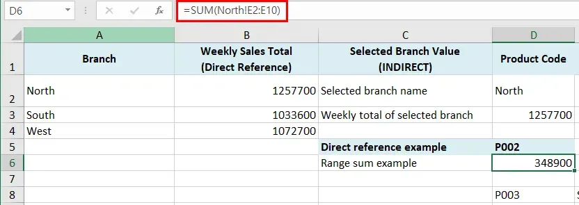
You'll often use ranges with functions like SUM or AVERAGE: =SUM(North!E2:E10).

Excel INDIRECT Function: Reference another sheet Dynamically

What is the INDIRECT Function?

=INDIRECT("SheetName!CellAddress") looks like a direct reference, but the sheet name is text. That means you can change which sheet you're pulling from using cell values.

Finding and Fetching Values from another sheet in Excel

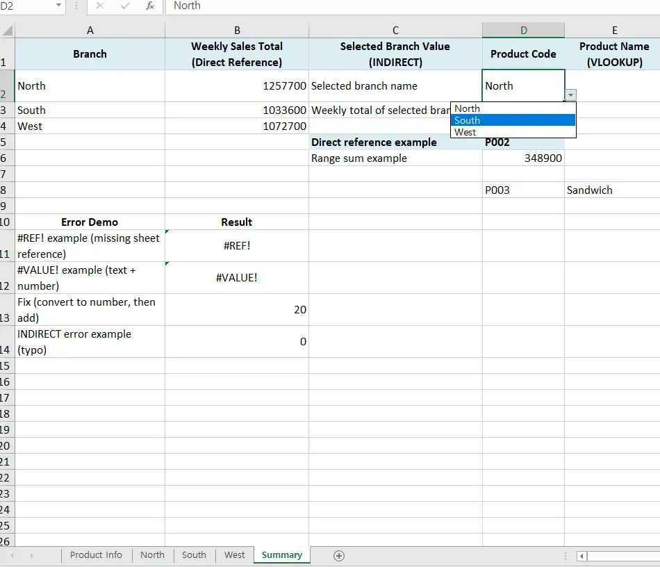
INDIRECT becomes truly powerful when you put the sheet name in a cell. For example, if you input "North" in a cell, data from the North sheet is automatically fetched.

How to Pull Data from Another Sheet Using INDIRECT

INDIRECT gets powerful when you put sheet names in cells.

If D2 says "North," INDIRECT pulls from the North sheet automatically.

=INDIRECT($D$2&"!H2") gets H2 from whatever sheet D2 names.

Type "North" in D2, and the formula pulls from North!H2.

Change D2 to "South", and it pulls from South!H2.

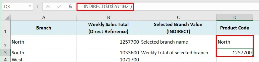
1. Put "North" in D2
2. Put =INDIRECT($D$2&"!H2") in another cell
3. Change D2 to "South" or "West"—watch the formula update

Excel INDIRECT: Get Multiple Values from another sheet

INDIRECT can also reference ranges.

=SUM(INDIRECT($D$2&"!B2:B10"))

This sums B2:B10 from whichever sheet D2 names. Add a dropdown in D2 and users can pick which sheet to pull from.

INDIRECT has some limitations:

• Workbooks must be open
• Heavy formulas with large datasets slow things down
• If you misspell a sheet name, you'll get a #REF! error.

Important: INDIRECT is a volatile function, meaning Excel recalculates it frequently.

In large workbooks, this can slow performance noticeably.

How to Use VLOOKUP to Reference Another Sheet in Excel

Excel VLOOKUP from Another Sheet: Formula Structure

Basic structure:

=VLOOKUP(lookup_value, OtherSheet!lookup_range, column_index, FALSE)

Lock your range with $ signs to prevent it from shifting when you copy the formula down.

Example—find unit prices from the Product Info sheet:

=VLOOKUP(B2,'Product Info'!$A$2:$C$9,3,FALSE)

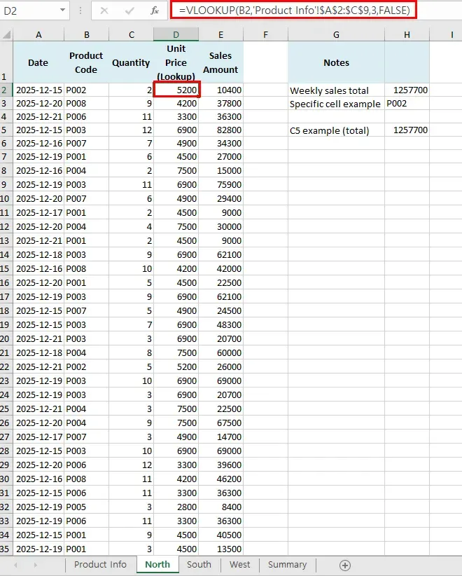
Here's what this formula does:

• B2: Product code you're looking up
• 'Product Info'!$A$2:$C$9: Search columns A-C on the Product Info sheet (locked range)
• 3: Return the value from column 3 (column C, Unit Price)
• FALSE: Exact matches only

Tip: If you’re using Microsoft 365 or Excel 2021+, consider XLOOKUP.

It’s more flexible than VLOOKUP and doesn’t break when columns are inserted or moved.

How to Check for Duplicates Against Another Sheet in Excel

You can use COUNTIF to check whether a value exists in a different sheet:

=COUNTIF(South!$B:$B, D8)

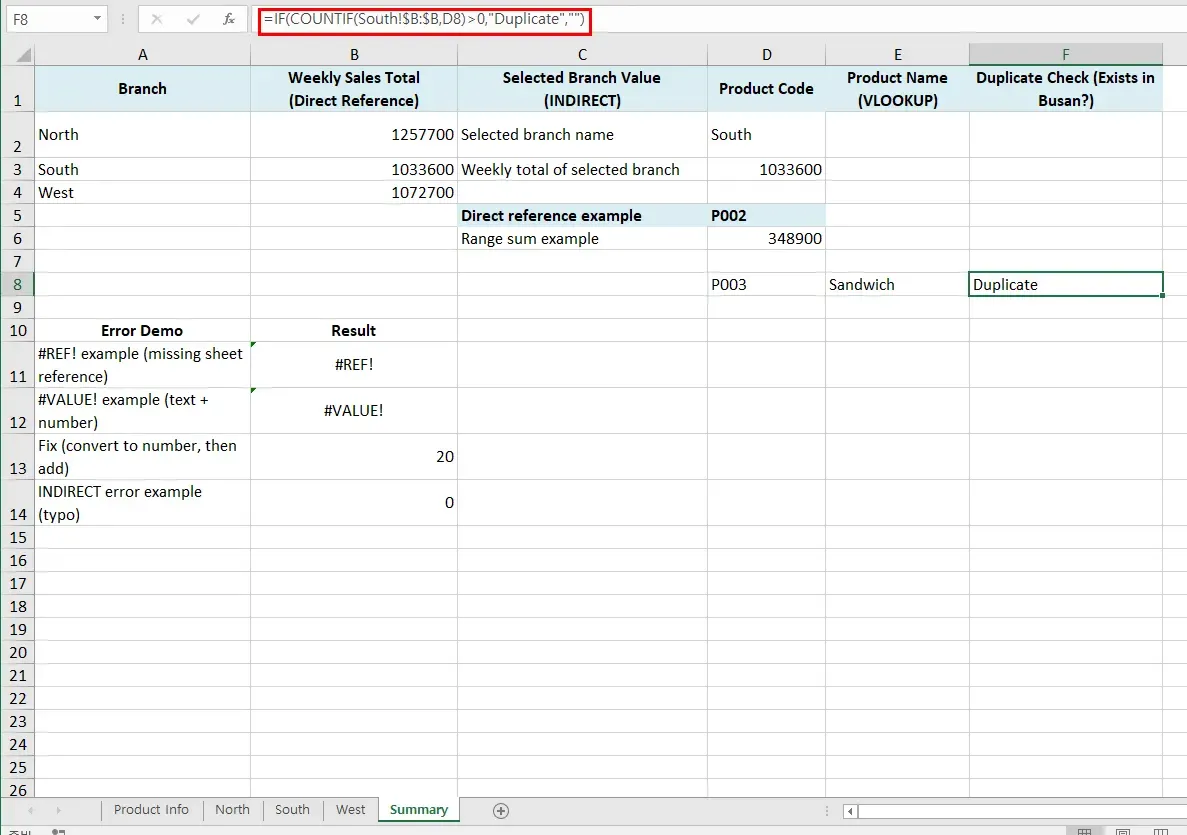
This counts how many times the value in D8 appears in the South sheet's column B. A result of 1 or more means the value exists in both sheets.

Show "Duplicate" when found:

=IF(COUNTIF(South!$B:$B,D8)>0,"Duplicate","")

To check against multiple sheets at once, combine conditions: =IF(OR(COUNTIF(South!$B:$B,D8)>0, COUNTIF(West!$B:$B,D8)>0),"Duplicate","")

How to Sum Values from Multiple Sheets in Excel

Excel Formula to Add Values from Different Sheets

To sum cells at the same position across multiple sheets, you can use the SUM function with multiple sheet references:

=SUM(North!H2, South!H2, West!H2)

This formula sums the H2 cell values from all three branch sheets. This way works well when you have just a few sheets.

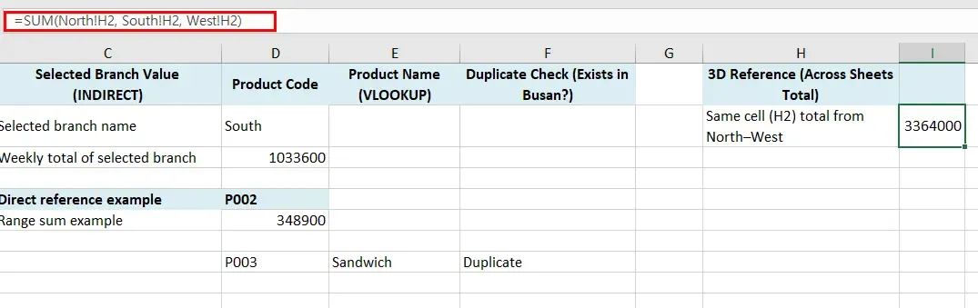
You can also use the + operator for simple cases, like =North!H2 + South!H2 + West!H2, but SUM keeps it cleaner as you add more sheets.

Excel 3D Reference: Sum the Same Cell Across Multiple Sheets

For consecutive sheets, 3D references are cleaner:

=SUM(Sheet1:Sheet3!A1)

Sums A1 from Sheet1 through Sheet3. Formula stays simple whether you have 3 sheets or 20.

Watch out: 3D references include everything between Sheet1 and Sheet3. If there's an extra sheet in the middle, it will be included in your calculation.

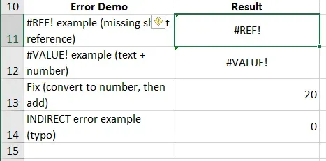
What Causes the #REF! Error?

#REF! means Excel can't find what you're referencing—usually from deleted or renamed sheets.

Excel #REF Error: Common Causes and Solutions

Why it happens:

• Deleted sheet: Formula points to a sheet that's gone
• Renamed sheet: Changed "SalesPerformance" to "2024Performance" but formulas still look for the old name
• Deleted cells: Removed rows or columns your formula needs

Fix it:

• Undo (Ctrl+Z): If you just deleted or renamed something, undo it immediately.
• Edit the formula: Click the error cell, fix the reference in the formula bar
• Find and Replace (Ctrl+H): Same error everywhere? Replace "SalesPerformance!" with "2026Performance!" in one shot

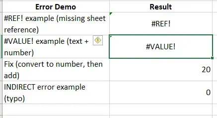
How to Fix #VALUE Error in Excel Cross-Sheet Formulas

#VALUE! means wrong data type in your formula.

Common causes:

• Bad sheet name in INDIRECT:
  A misspelled or missing sheet name can return #REF! (and sometimes #VALUE!, depending on context)
• Text in math: Sheet2!A1 has "Sales" but you're trying =Sheet2!A1 + 10
• Text dates: Date math fails when dates are stored as text

Solutions:

• Double-check sheet names in INDIRECT
• Verify what's in referenced cells—use VALUE() to convert text to numbers
• Strip hidden spaces with =TRIM(Sheet2!A1)

How to Prevent Excel Formulas from Breaking When Copying

Why Cross-Sheet References Frequently Break

References break in real work from structural changes—here's what causes it.

Common Reasons Excel References Break Across Sheets

• Rearranged sheets: 3D references give wrong results when you reorder sheets
• Copied sheets: Duplicating a sheet copies its formulas, but relative references might point somewhere unexpected—lock ranges with =VLOOKUP(A2, Sheet2!$A$1:$C$10, 2, FALSE)
• Moved files: Move a workbook that links to others and references break
• Team edits: Someone deletes or renames a sheet while you're working

How to Create Hyperlinks Between Sheets in Excel

Referencing sheets links data.

Hyperlinks are for navigation—they help you jump between sheets quickly without pulling values.

Excel Hyperlinks: Navigate Between Sheets Quickly

Beyond data referencing, you can create hyperlinks for quick navigation between sheets. This is useful when there are many sheets.

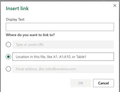
1. Click a cell
2. Hit Ctrl+K (or right-click > Link)
3. Select Location in this file (e.g., A1, A1:A10, or Table1)
4. Type the cell address and choose your sheet
5. Click OK

Click the cell and you jump straight there.

Best Practices for Excel Cross-Sheet References

Here's what works best in professional settings.

Direct references for straightforward pulls. =Sheet2!A1 is fastest and most reliable. Less can go wrong, better performance.

INDIRECT for dynamic switching. Users picking different sheets (monthly reports, quarterly summaries)? INDIRECT handles it.

VLOOKUP for data lookups. Finding specific information based on criteria rather than just grabbing a cell? Use VLOOKUP or XLOOKUP.

3D references for multi-sheet totals. =SUM(Sheet1:Sheet12!A1) sums the same cell across consecutive sheets cleanly.

Lock ranges with $. Stop formulas from shifting when you copy them down.

Think through your structure. Keep source sheets separate from summaries. Don't rename sheets after formulas are set up.

Stop Writing Cross-Sheet Formulas. Let Cicely AI Handle Your Multi-File Workflow.

You've learned how to reference data across sheets manually. But what about when you need to consolidate 50 Excel files, cross-reference data from PDFs, and clean messy formats all at once?

Cicely AI is a desktop-native AI coworker built specifically for Excel users who work with complex, multi-file workflows. Instead of manually writing VLOOKUP formulas, building INDIRECT references, and troubleshooting #REF! errors, Cicely works directly inside your Excel workbooks on your computer.

Unlike ChatGPT or web-based tools, Cicely doesn't require uploading or copy-pasting between applications. Tell Cicely what you need in plain English: "Merge data from these 20 branch files," "Cross-reference customer IDs with the pricing sheet," or "Clean this data and remove duplicates." Cicely scans your local files, consolidates everything, and delivers analysis-ready spreadsheets while you review each change before it applies.

Everything runs locally on your PC. No file uploads. No browser tools.