How to Use VLOOKUP in Excel: Examples, Exact Match, and #N/A Fixes

Have you ever seen an Excel sheet where entering an employee number automatically displays their name and department, or typing a product code instantly shows the price and inventory?

You can build this kind of lookup behavior with VLOOKUP.

However, many users encounter incorrect values or #N/A errors because the table_array range shifts, or because the TRUE/FALSE match setting is wrong.

This guide walks you through the Excel VLOOKUP function from its basic structure to the most common mistakes in real-world applications.

What is the Excel VLOOKUP Function?

VLOOKUP searches the leftmost column of a table and returns a value from another column in the same row.

In short, it's a tool that automatically looks up information by entering a specific ID, code, or name.

In day-to-day work, VLOOKUP is commonly used to pull details such as an employee’s name or department from an ID, or a product’s price and specs from a product code.

One key rule: The lookup value must be located in the leftmost column of the table range, and the results to retrieve must always be in columns to the right. VLOOKUP can only return values to the right of the lookup column.

How to Use VLOOKUP in Excel: The 4 Arguments Explained

To understand how to use VLOOKUP in Excel, you need to know the four arguments precisely. The basic structure of the function is =VLOOKUP(lookup_value, table_array, col_index_num, range_lookup).

First Argument: lookup_value (Value to Find)

This is the reference value that determines what you're looking for. You specify the lookup criteria such as employee number 1001, customer number C-023, or product code P002. If you're finding a score by entering a student's name in a grade sheet, the student's name becomes the lookup_value.

Second Argument: table_array (Search Range)

This is the table range where you'll search. The important point here is that the reference column (the column containing lookup_value) must be the first column of this range. If you're finding information by employee number, the employee number column must be positioned at the far left of the table_array.

Third Argument: col_index_num (Column Number)

This is the number indicating which column's value to retrieve from the table. The first column of table_array is 1, followed by 2, 3, 4 to the right. For example, if the employee number is in the first column and the name is in the second column, you enter 2 to retrieve the name.

Fourth Argument: range_lookup (Match Option)

This option determines whether to find only exact matches or allow approximate values. FALSE (or 0) finds only exact matches, while TRUE (or 1) finds approximate values. If you omit this argument, Excel defaults to TRUE (approximate match). For most lookups (IDs, product codes, emails), always use FALSE.

VLOOKUP Example Excel - Employee Information Lookup

Let's practice how to use VLOOKUP in Excel with a real VLOOKUP example Excel scenario. In the Employee_List sheet, columns A through D contain employee number, name, department, and phone number. We'll create a setup where entering an employee number in the Lookup_Form sheet automatically displays the name and department.

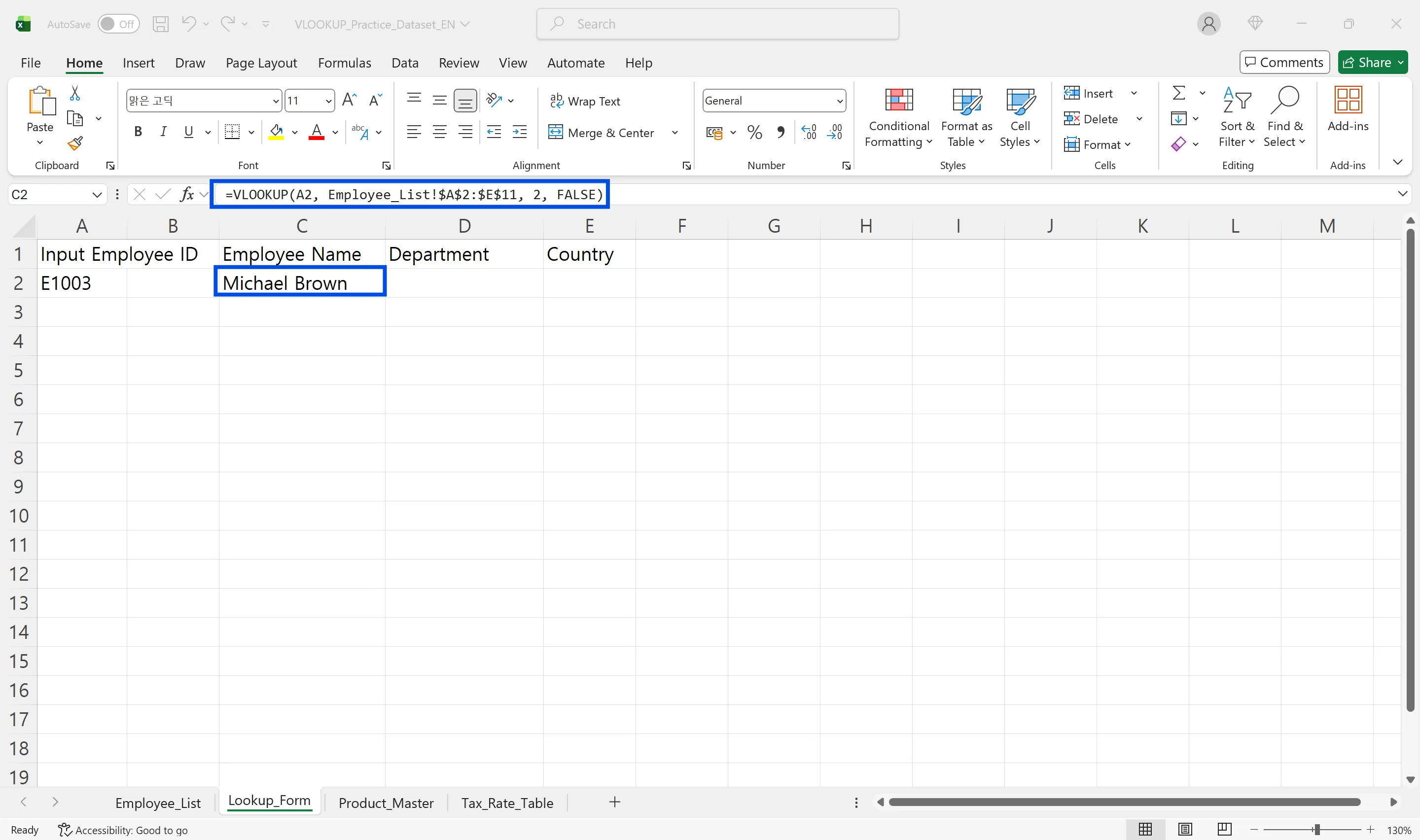
Creating the Name Retrieval Formula

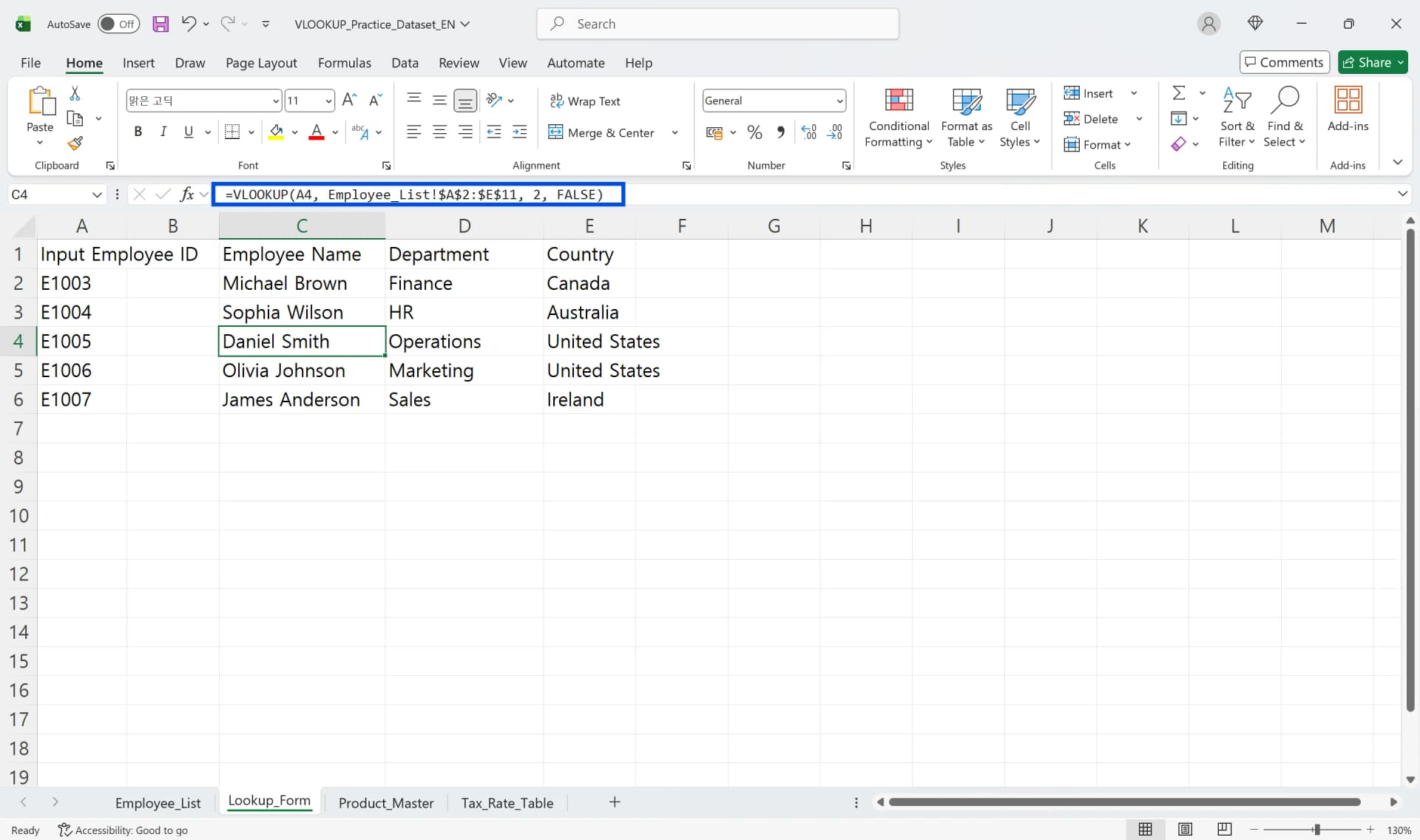
1. Enter the employee number in cell A4 of the Lookup_Form sheet.
2. In cell C4 (name display location), type the following formula: =VLOOKUP($A$4, Employee_List!$A$2:$D$11,2, FALSE)
3. The value 2 is used for col_index_num because Full Name is stored in the second column of the Employee_List table (column B).
4. Press Enter, and the employee name corresponding to the entered ID will appear.

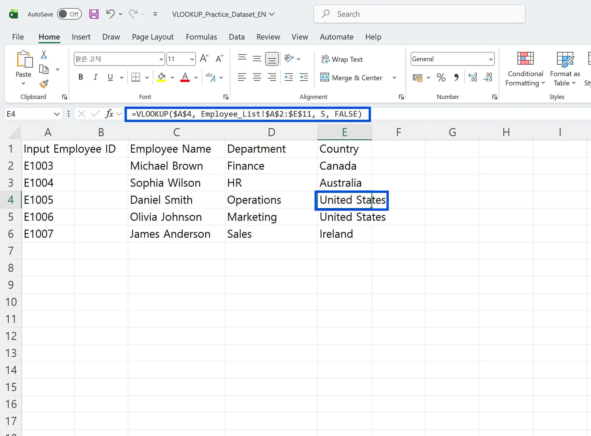
Creating the Department Retrieval Formula

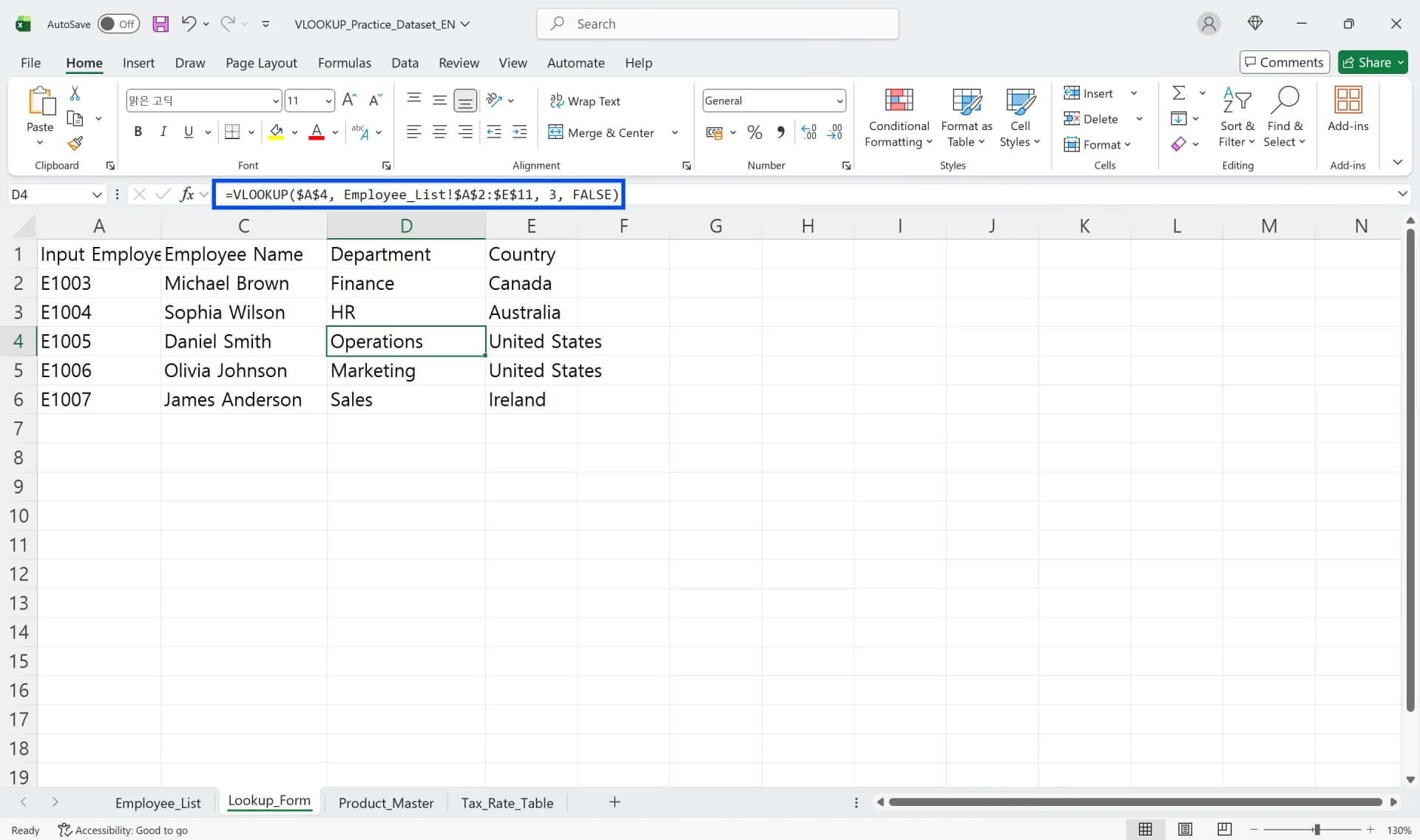
1. In cell D4 (department display location), enter: =VLOOKUP($A$4, Employee_List!$A$2:$D$11,3, FALSE)
2. Here, 3 refers to the third column of the table array, which contains department information (column C).
3. When copying the formula down, it is recommended to fix the table_array range using absolute references to prevent reference shifting.

Use VLOOKUP Across Sheets (Cross-Sheet References)

This VLOOKUP example Excel demonstrates how to use VLOOKUP multiple sheets Excel.

The formula references data from a different sheet by including the sheet name followed by an exclamation mark, such as Employee_List!$A$2:$D$11. This allows you to retrieve information across multiple sheets within the same workbook while working in a separate lookup form.

3 Most Common VLOOKUP Mistakes in Real-World Use

When learning how to use VLOOKUP in Excel, even one incorrect setting can distort data or cause #N/A errors. Here are the three most frequent mistakes in real-world applications.

Mistake 1: Not Fixing Range with Absolute References

When copying VLOOKUP formulas right or down, the cell addresses in table_array shift together, causing problems by referencing the wrong range. For example, if the employee list table is A2:D100 and you copy the formula down, it shifts to A3:D101, missing the last employee's information.

To prevent this, you must fix table_array with absolute references as $A$2:$D$100. Press F4 to add dollar signs or type them directly. Only with a fixed range will the formula always reference the same table when copied.

Mistake 2: Confusing range_lookup TRUE/FALSE

Omitting or incorrectly setting the fourth argument range_lookup produces wrong values. In Excel, leaving this argument blank applies TRUE as the default, activating approximate match mode. When finding values that must match exactly like employee numbers or product codes, using TRUE can retrieve similar values without you realizing the mistake.

For most business lookups like employee information, product masters, and customer data, you must use FALSE. TRUE is only used when determining which bracket a value falls into, like tax brackets or grade ranges. In real work, habitually specifying FALSE is the safe approach.

Mistake 3: Incorrectly Specifying col_index_num

Some people forget that table_array's first column starts at 1 and counts to the right, confusing it with Excel sheet column numbers (A=1, B=2). For example, if table_array is range C:F, then column C is 1, column D is 2, column E is 3, and column F is 4.

Also, #N/A errors can occur when the lookup value simply does not exist in the first column, or when you select only part of the data and copy down with the fill handle, leaving newly added rows outside the range. When specifying ranges, generously include all data or use Ctrl+T to create a table for automatic expansion.

VLOOKUP Exact Match Excel - TRUE vs FALSE Explained

The range_lookup argument is the most frequently misunderstood part when learning how to use VLOOKUP in Excel. You must clearly understand the difference between FALSE and TRUE to properly utilize VLOOKUP exact match Excel capabilities.

VLOOKUP Exact Match Excel: FALSE (0)

VLOOKUP exact match Excel mode with FALSE finds values in table_array's first column that exactly match lookup_value. If not found, it returns a #N/A error. Almost all general employee information, product masters, and customer data lookups must use FALSE for exact matching. You can't retrieve employee number 1000 or 1002 when looking for employee number 1001.

Approximate Match: TRUE (1)

TRUE finds the largest value that is less than or equal to the lookup value. This mode requires the first column to be sorted in ascending order to work properly. It's useful when determining which range a value falls into.

For example, assume you have a tax bracket table. If column A has taxable income thresholds (0, $12,000, $46,000, etc.) and column B has tax rates (6%, 15%, etc.), the formula =VLOOKUP(D2, $A$2:$B$6, 2, TRUE) automatically finds which bracket the taxable income falls into and retrieves the tax rate.

TRUE is also used for assigning grades. Create a table with score ranges (0, 60, 70, 80, 90) and grades (F, D, C, B, A), and finding which range a student's score falls into automatically assigns the grade. However, column A's score ranges must be sorted in ascending order.

The Trap of TRUE Being the Default

Many users think they can omit the fourth argument, only to get wrong values later. This is because Excel internally applies TRUE when range_lookup is left blank. When using VLOOKUP exact match Excel, always specify FALSE explicitly to ensure accurate results.

VLOOKUP Limitations and Alternatives

The Excel VLOOKUP function is powerful but has several limitations. Understanding these and knowing alternatives helps you handle more complex situations.

Limitation of Only Searching Left Columns

VLOOKUP requires the lookup value to be in table_array's leftmost column. If the desired result is to the left of the reference column, VLOOKUP cannot do it. In this case, combine INDEX and MATCH functions, or use the XLOOKUP function in recent Excel versions to find values regardless of column order.

INDEX/MATCH is more flexible because it can look up values in any direction—and your formula won’t break if columns move. It's a method of specifying the range to retrieve with the INDEX function and finding which row with the MATCH function. You don't need to rearrange columns, and you can look up left columns.

Difficulty Handling Multiple Criteria

VLOOKUP basically uses only one condition (lookup_value). If you want to find a phone number that simultaneously matches name and department, you need multiple criteria processing. In this case, create a helper column to generate a unique key combining name and department, or use SUMIFS or INDEX/MATCH combinations.

Problems with Duplicate Values

VLOOKUP searches from top to bottom and returns only the first value found. If there are people with the same name, it only retrieves the first person's information. To prevent this, use unique key values (like employee numbers) or normalize data without duplicates.

How to Use VLOOKUP in Excel - Frequently Asked Questions

Q. Why do I get #N/A errors when using VLOOKUP?

#N/A errors occur when lookup_value and the values in table_array's first column don't match exactly. It's often due to invisible spaces (leading/trailing spaces) or differences between number and text formats. Remove spaces with the TRIM function or unify formats with VALUE or TEXT functions to resolve this.

Q. Should I use TRUE or FALSE for VLOOKUP exact match Excel?

In most real-world situations, use FALSE for VLOOKUP exact match Excel. When you must find exact matches like employee numbers, product codes, or customer numbers, you must specify FALSE. TRUE is only used when determining which bracket a value falls into, like tax brackets or grade ranges, and in this case, the first column must be sorted in ascending order.

Q. How do I use VLOOKUP multiple sheets Excel?

To use VLOOKUP multiple sheets Excel, include the sheet name followed by an exclamation mark before the cell range in your table_array argument. For example: =VLOOKUP(A2,'SheetName'!A:D,2,FALSE). This allows you to pull data from any sheet in your workbook.

Q. Why are absolute references necessary in VLOOKUP?

When copying VLOOKUP formulas, if the table_array range shifts together, it references the wrong data. Setting absolute references as $A$2:$D$100 ensures the formula always references the same range no matter where you copy it, preventing errors.

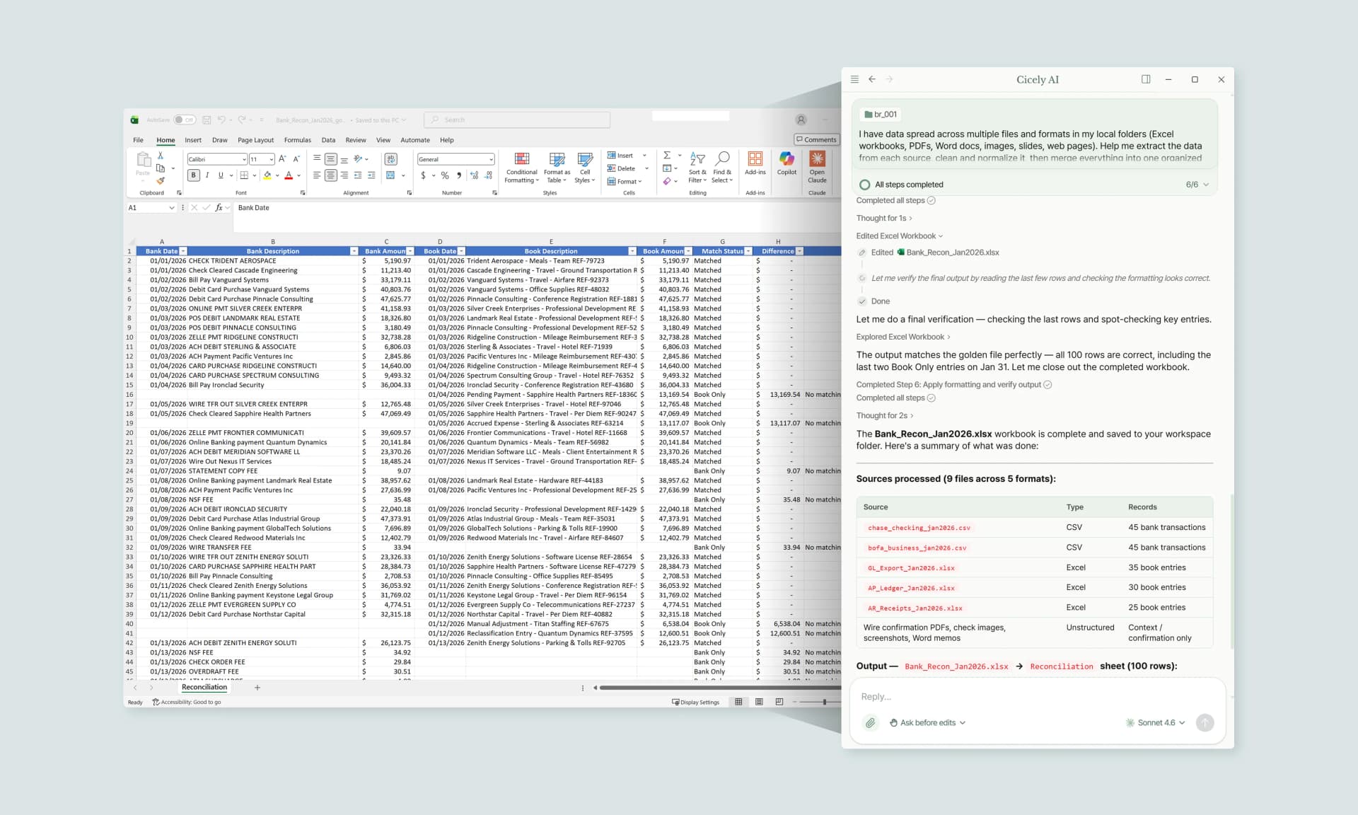
Work More Efficiently in Excel with Cicely AI

VLOOKUP is simple once you know the rules, but real worksheets still create friction: fixing ranges, checking exact match settings, and tracking down #N/A errors.

Cicely AI is a desktop-native AI coworker for Excel. Tell Cicely what you need in plain English, such as “Create a VLOOKUP that returns department by employee ID” or “Explain why this formula returns #N/A,” and review the suggested steps. Everything runs locally on your PC, with no file uploads.